Medical Cost Prediction

A machine learning approach to predict medical costs from demographic and health inputs

Introduction

The goal of this notebook is to characterize the dataset and ultimately help predict medical charges based on factors like age, sex, bmi, number of children, smoking status, and region of living.

Let us start with loading the necessary packages for this analysis.

packages <- c("shiny", "tidyverse", "lubridate", "randomForest", "plotly",
              "ggstatsplot", "corrplot", "Hmisc", "flextable", "DT", "networkD3",
              "ggrepel", "leaflet", "maps", "ggforce", "lmtest", "ggpubr")
installed_packages <- packages %in% rownames(installed.packages())
if (any(installed_packages == FALSE)) {
  install.packages(packages[!installed_packages])
}
invisible(lapply(packages, library, character.only = TRUE))


library(shiny)
library(tidyverse)
library(lubridate) 
library(randomForest)
library(plotly)
library(ggstatsplot)
library(corrplot)
library(Hmisc)
library(flextable)
library(DT)
library(networkD3)
library(ggrepel)
library(leaflet)
library(maps)
library(ggforce)
library(lmtest)
library(ggpubr)

karl_theme <- theme_bw() +
  theme(plot.title = element_text(size=20),
        axis.title = element_text(size = 15),
        axis.text = element_text(size = 12),
        legend.title = element_text(size=12),
        legend.text = element_text(size=12))

Data Upload and Clean-up

medicalcost <- read.csv("medical_cost.csv")
medicalcost <- medicalcost %>% 
  mutate(BMI.status = case_when(
    bmi < 18.5 ~ "Underweight",
    bmi >= 18.5 & bmi < 24.9 ~ "Normal",
    bmi >= 25 & bmi < 29.9 ~ "Overweight",
    bmi >= 30 ~ "Obese",
    TRUE ~ "Unknown")) %>%
  mutate(BMI.status = factor(BMI.status, ordered = TRUE,
                             levels = c("Underweight", "Normal", "Overweight", "Obese", "Unknown"))) %>% 
  mutate(children = factor(children, 
                           ordered = TRUE,
                           levels = c("0", "1", "2", "3", "4", "5"))) %>% 
  mutate(sex = factor(sex, ordered = TRUE, levels = c("male", "female"))) %>% 
  mutate(smoker = factor(smoker, ordered = TRUE, levels = c("no", "yes"))) %>% 
  mutate(region = factor(region, ordered = TRUE, levels = c("northeast", "northwest", "southeast", "southwest")))

I added a variable to stratify the BMI into 4 different categories: Underweight, Normal, Overweight, and Obese. I also transformed the sex, bmi status, children, smoking status, region into categorical factors. The resulting data frame is as follows:

medicalcostinfo <- medicalcost %>% 
  datatable(
    filter = list(position = "top", clear = FALSE),
    options = list(columnDefs = list(list(className = "dt_center", targets = "_all")),
                   scrollX = TRUE),
          caption = "Medical cost dataset"
        )
medicalcostinfo

Exploratory Data Analysis

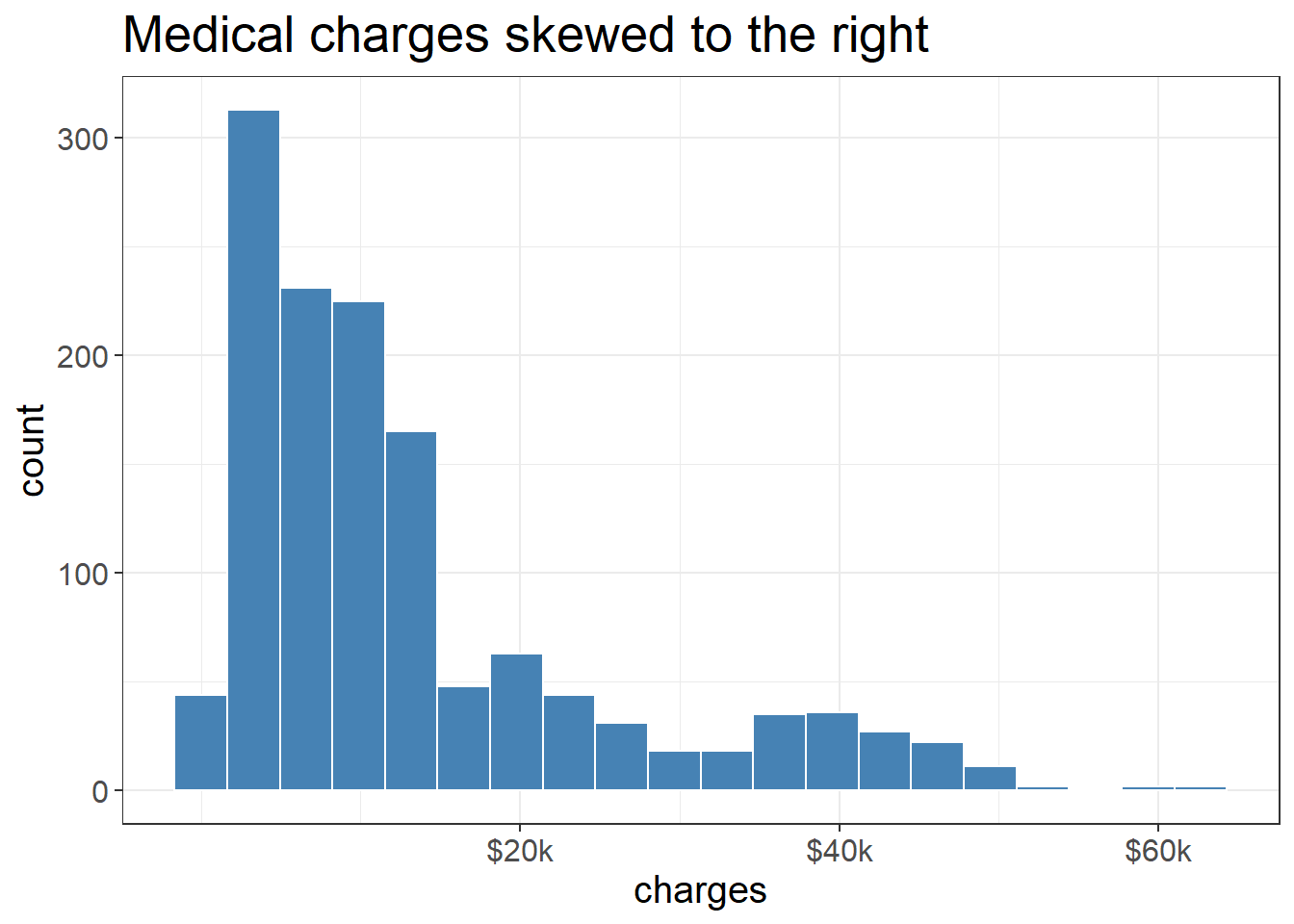
Distribution of medical charges in the data set

ggplot(medicalcost, aes(x = charges)) +
  geom_histogram(bins = 20, fill = "steelblue", color = "white") +
  labs(title = "Medical charges skewed to the right") +
  scale_x_continuous(breaks = c(20000, 40000, 60000),
                     labels = c("$20k", "$40k", "$60k")) +
  karl_theme

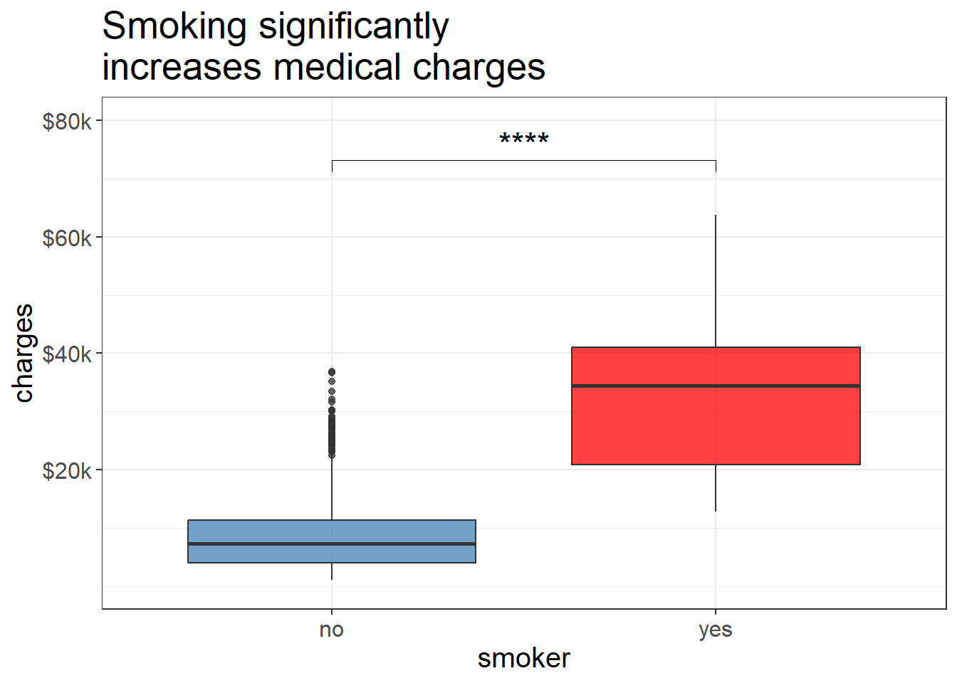
Smokers have higher medical cost than non-smokers

smoking.comparison <- list(c("yes", "no"))

ggplot(data = medicalcost, aes(x = smoker, y = charges, fill = smoker)) +
  geom_boxplot(alpha = 0.75) +
  labs(title = "Smoking significantly\nincreases medical charges") +
  scale_fill_manual(values = c("yes" = "red", "no" = "steelblue")) +
  stat_compare_means(comparisons = smoking.comparison, 
                     aes(label = ..p.signif..), 
                     label.y = 70000, size = 6) +
  karl_theme +
  theme(legend.position = "none") +
  scale_y_continuous(limit = c(0, 80000),
                     breaks = c(20000, 40000, 60000, 80000),
                     labels = c("$20k", "$40k", "$60k", "$80k"))

Unpaired T test suggests that smokers have higher cost of medical charges than non-smokers. How does these two groups affect the medical cost with a third variable, such as age and BMI?

Relationship between age and medical cost

ggplot(medicalcost, aes(x = age, y = charges, color = smoker)) +
  geom_point(alpha = 0.75, size = 2.5) +
  scale_color_manual(values = c("yes" = "red", "no" = "steelblue")) +
    labs(title = "Older smokers are associated\nwith higher medical charges") +
  scale_y_continuous(breaks = c(20000, 40000, 60000),
                     labels = c("$20k", "$40k", "$60k")) +
  karl_theme

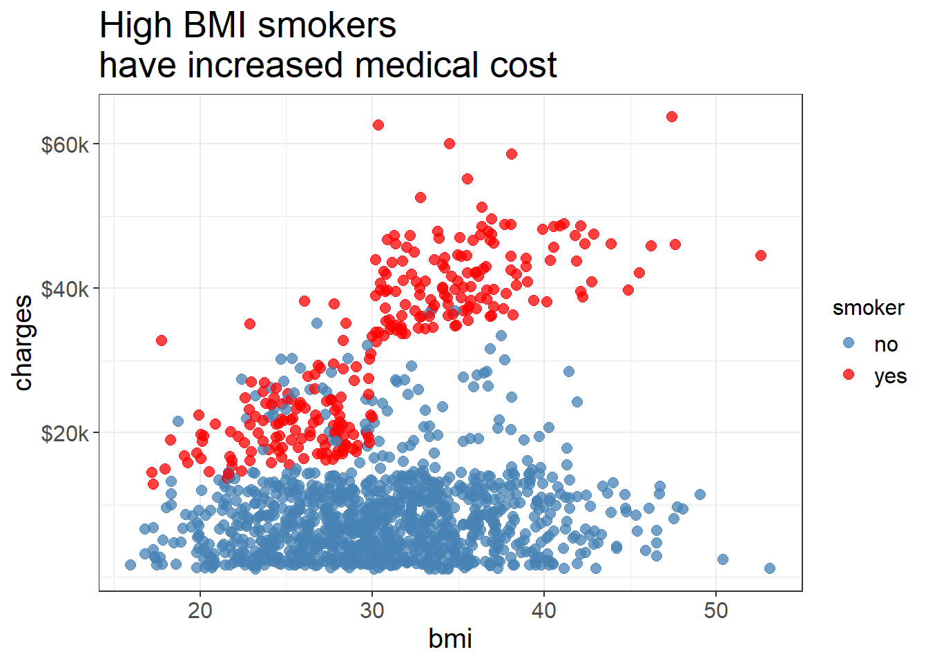
Relationship between BMI and medical cost

ggplot(medicalcost, aes(x = bmi, y = charges, color = smoker)) +
  geom_point(alpha = 0.75, size = 2.5) +
  scale_color_manual(values = c("yes" = "red", "no" = "steelblue")) +
    labs(title = "High BMI smokers\nhave increased medical cost") +
  scale_y_continuous(breaks = c(20000, 40000, 60000),
                     labels = c("$20k", "$40k", "$60k")) +
  karl_theme

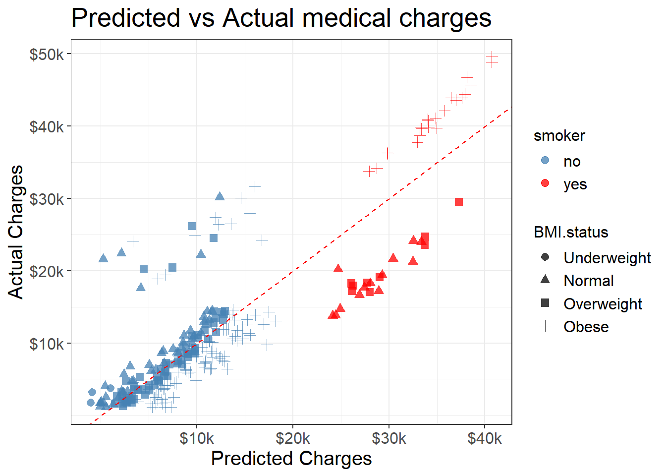
Model using Multiple Linear Regression

Perform modeling using training set using 80% of the data

set.seed(123)
sample_index <- sample(seq_len(nrow(medicalcost)), size = 0.8 * nrow(medicalcost))
train_data <- medicalcost[sample_index, ]
test_data <- medicalcost[-sample_index, ]

model <- lm(charges ~ age + bmi + smoker, data = train_data)
summary(model)

Call:
lm(formula = charges ~ age + bmi + smoker, data = train_data)

Residuals:
     Min       1Q   Median       3Q      Max 
-12468.6  -3091.6   -920.8   1721.2  28807.8 

Coefficients:
            Estimate Std. Error t value Pr(>|t|)    
(Intercept)   283.34    1076.80   0.263    0.793    
age           245.79      13.70  17.939   <2e-16 ***
bmi           341.34      31.27  10.917   <2e-16 ***
smoker.L    17081.13     325.82  52.424   <2e-16 ***
---
Signif. codes:  0 '***' 0.001 '**' 0.01 '*' 0.05 '.' 0.1 ' ' 1

Residual standard error: 6179 on 1066 degrees of freedom
Multiple R-squared:  0.7494,    Adjusted R-squared:  0.7487 
F-statistic:  1063 on 3 and 1066 DF,  p-value: < 2.2e-16

According to the model:

• For every additional increase in age, medical cost increases by $245.79.
• For every unit increase in BMI, cost increases by $341.34.
• Smokers are expected to cost $17k more than non-smokers, on average.

Test the model using 20% of the data

test_data$predicted <- predict(model, newdata = test_data)
test_data <- test_data %>% 
  filter(BMI.status != "Unknown")

ggplot(test_data, aes(x = predicted, y = charges, color = smoker, shape = BMI.status)) +
  geom_point(alpha = 0.75, size = 2.5) +
  scale_color_manual(values = c("yes" = "red", "no" = "steelblue")) +
  geom_abline(slope = 1, intercept = 0, color="red", linetype="dashed") +
  labs(title = "Predicted vs Actual medical charges",
       x = "Predicted Charges", y = "Actual Charges") +
  scale_y_continuous(breaks = c(10000, 20000, 30000, 40000, 50000),
                     labels = c("$10k", "$20k", "$30k", "$40k", "$50k")) +
  scale_x_continuous(breaks = c(10000, 20000, 30000, 40000),
                     labels = c("$10k", "$20k", "$30k", "$40k")) +
  karl_theme

In our model testing, we see that the model underestimates actual medical charges for smoking obese demographic.